Attention in Transformers - An overview
Overview
- Similarity between words
- Dot product
- Cosine similarity
- The Key, Query, Value matrices as linear transformations
Words are made as word embeddings (numerical values) Context helps to determine what kind of word that should refer to. This is where similarity comes in.
Dot product
Think of a 2D graph with x and y axes. The dot product is a multiplication of the words in matrix form (matrix multiplication). eg. [2, 3] * [1, 4]-> (2 * 1) + (3 * 4) = 14 The first one times the transpose of the second one
Cosine Similarity
points on the graph are traced to the origin and the angle is gotten using the arctan property and the angle is put into the cosine() function to give the value.
Scaled Dot product
The answer from the dot product divided by the length of the vector. eg. 14/sqrt(2) This helps to prevent the exploding gradient problem.
Normalization
After the word math step, the words should be normalized/scaled down to prevent the use of extremely large numbers. The softmax activation function is used.
Keys and Queries
Turn the embedding into one that is best for calculating similarities.
Values
Best embedding for finding the next word. Multiplies the embedding from the keys and queries and multiplies it by itself.
Why move words on a different embedding?
The first can give info like:
- color
- size
- high level embeddings
The second one (values) knows when two words could appear in the same context.
Multi-Head Attention
Many heads are used (n-times). basically the single head attention procedure is done many times.
Concatenating
If you have an embedding of 3 (2 dimensions) you get 6 dimensions
Linear step
It transforms the dimensions into lower ones which could actually be used. The best ones are scaled up, the worst are scaled down. Then an optimal embedding is produced.
The Math
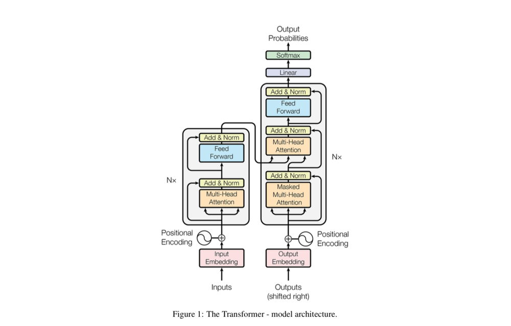
Starting with the encoder
Input imbedding:
- A sentence of words are tokenized (split into single words).
- The words are then mapped into numbers that represent the position of words in our vocabulary. Numbers(input ID) are mapped into a vector of 512 numbers.
- The same word gets mapped to the same embedding.
- The numbers (embeddings) are changed by the model and hence are not fixed.
- They change according to the needs of the loss function.
Positional Encoding:
- Each word should carry information about its pos in the sentence.
- That is what positional encoding does.
- Words closer to each other as "close" and those distant from each other as "distant".
- $$PE(ps, 2i) = \sin(pos\10000^{2i\d} )$$
- $$PE(pos, 2i+1) = \cos(pos\10000^{2i\d})$$
- Positional encodings are computed once and reused.
- Trigonometric functions represent a pattern the model can recognize as continuous, so relative positions are easier to see for the model.
Self-Attention:
- it allows the model to relate words to each other
- $$Attention(Q, K, V) = softmax(\frac{QK^{T}}{\\sqrt{ d }})V$$
- d = 512 / len(seq); T=transpose
- softmax keeps the values between 0 and 1 (they sum up to 1)
Multi-Head Attention: $$ Multihead(Q, K, V) = Concat(head_{1}\dots.head_{n})W $$ $$ head_{i} = Attention(QW_{i}^{Q}, KW_{i}^{K}, VW_{i}^{V}) $$
Layer Normalization:
- normalize to make new values in the range 0-1
- beta and gamma parameters are added
- model learns from this parameters to amplify values that need amplification
For the decoder:
Masked Multi-Head:
- prevent model from seeing future words
- replace the future values with -inf
- the softmax sends the -inf to a very small value -> 0
- this is done after the matmul, just before the softmax function